Introduction
The multi-commodity flow problem is a network flow problem with multiple commodities. Given a directed graph and a set of commodities, the goal is to find a flow for each edge and each commodity such that the flow satisfies the capacity constraints of the edges and the conservation of flow at each node. Even though the demands are different, the capacities of the edges are often shared between the commodities, which poses a challenge in finding a feasible solution.
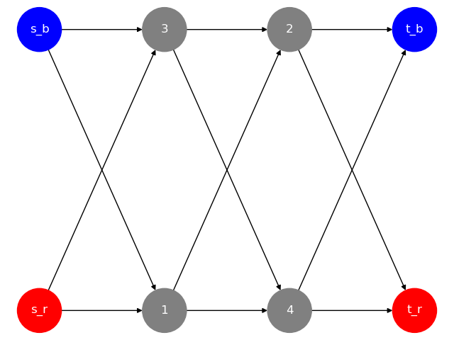
In the example above, we have a directed graph with two commodities which are represented by two sets of source and sink nodes: red and blue.
The multi-commodity flow problem can are applicable in various domains such as transportation, telecommunication, and logistics. For example:
- In transportation, the multi-commodity flow problem can be used to model the fact that multiple different vehicles are traveling on the same road network. The utilization of the road network is different between buses, cars, and trucks due to their different sizes and weights.
- In telecommunication, the multi-commodity flow problem can be used to model the fact that different types of data are transmitted over the same network. The bandwidth requirements of video, audio, and text data are all different due to their different sizes, formats and consumption patterns.
In 2021, Liu et al proposed a localized solution method for the multi-commodity flow problem. The method is a combinatorial algorithm that are localized in the sense that it looks at each edge and node in isolation at each iteration. Furthermore, the authors showed that the algorithm will always converge to an optimal solution if it exists. As such the algorithm promises an exact solution for the multi-commodity flow problem that is also highly parallelizable, which is worth exploring.
Mathematical notations
Much like the single-commodity flow problem, the multi-commodity flow problem can be formulated as a linear program. The multi-commodity flow problem can be defined with the following constraints:
-
The sum of the flow for all commodities on each edge must be less than or equal to the capacity of the edge:
\[ \sum_{k \in \mathcal{K}} f_{ij,k} \leq u_{ij}, \quad \forall (i, j) \in E \]
-
The flow for all commodities at each node must be conserved, except for the source and sink nodes of each commodity.
\[ \sum_{j \in \delta^+(i)} f_{ij,k} - \sum_{j \in \delta^-(i)} f_{ji,k} = \hat{\Delta}_{ik}, \quad \forall k \in \mathcal{K}, ; i \in V \]
where \( \hat{\Delta}_{ik} \) is defined as:
\[ \hat{\Delta}_{ik} = \begin{cases} 0, & \text{if } i \in V \setminus \{s_k, t_k\} \\ d_k, & \text{if } i = s_k \\ -d_k, & \text{if } i = t_k. \end{cases} \]
-
The flow for all commodities on each edge must be non-negative.
\[ f_{ij,k} \geq 0, \quad \forall k \in \mathcal{K}, \quad (i, j) \in E \]
Here, we have:
- \(\mathcal{K}\) is the set of all commodities.
- \(V\) is the set of all nodes.
- \(E\) is the set of all edges.
- \(f_{ij,k}\) is the flow on edge \((i, j)\) for commodity \(k\).
- \(u_{ij}\) is the capacity of edge \((i, j)\).
- \(d_k\) is the demand of commodity \(k\).
- \( \hat{\Delta}_{ik} \) is a correction term used to account for the added or removed flow at the source and sink nodes of each commodity.
- \(\delta^+(i)\) and \(\delta^-(i)\) are the sets of edges that are incident to node \(i\) in the forward and backward directions, respectively.
Relaxation
The main idea of the algorithm devised by Liu et al is to relax both the conservation of flow constraint on the vertices and the capacity constraint on the edges. This relaxation is done by introducing a pseudo-flow.
The pseudo-flow, defined as \( \mathcal{f}: K \times E \to \mathbb{R}^+ \), is a function that maps each commodity \( k \in \mathcal{K} \) and edge \( (i, j) \in E \) to a non-negative real number, which is just the same as that of a real flow. The main difference is that the pseudo-flow does not need to satisfy the constraints noted above.
Going forward, all \( f_{ij,k} \) will refer to the pseudo-flow unless otherwise noted.
Height
Relaxing the conservation of flow constraint on the vertices, we keep track of the amount by which the flow going into a vertex exceeds the flow going out of it:
\[ \Delta_{ik} = \sum_{j \in \delta^-(i)} f_{ji,k} - \sum_{j \in \delta^+(i)} f_{ij,k} + \hat{\Delta}_{ik}, \quad \forall i \in V, ; k \in \mathcal{K} \]
We now refer to this as the height of the vertex \( i \) for commodity \( k \).
\[ h_{ik} = \Delta_{ik} \]
We can see that the conservation of flow constraint will hold when the height of all vertices is zero.
Congestion
Relaxing the capacity constraint on the edges, we keep track of the amount by which the flow on an edge exceeds its capacity:
\[ \psi_{ij} = \begin{cases} f_{ij} - u_{ij}, & \text{if } f_{ij} > u_{ij} \\ 0, & \text{if } f_{ij} \leq u_{ij} \end{cases} \]
where \(f_{ij}\) is just the sum of the pseudo-flows for all commodities on edge \((i, j)\):
\[ f_{ij} = \sum_{k \in \mathcal{K}} f_{ij,k} \]
We can see that the capacity constraint will hold when the congestion of all edges is zero.
Potential difference
Now that we have defined the height and congestion, we can define the potential difference for each commodity \( k \in \mathcal{K} \) between two vertices \( i \) and \( j \):
\[ \phi_{ij,k} = h_{ik} - h_{jk} - \psi_{ij} \]
Intuitively, if the potential difference is positive, it means that the flow from \( i \) to \( j \) for commodity \( k \) is too low because of broken conservation of flow.
Conversely, if the potential difference is negative, it means that the flow from \( i \) to \( j \) for commodity \( k \) is too high because of broken conservation of flow or capacity constraint.
As noted, for both the flow conservation and capacity constraints to hold, all heights and congestions must be zero, which implies that the potential difference must be zero for all commodities on all edges in a feasible solution.
However, the converse is not necessarily true. A zero potential difference does not imply that the flow is feasible. This is because we could have a positive \( h_{ik} - h_{jk} \) (more flow going into \( i \) than going out of \( j \)) and a positive \( \psi_{ij} \) (flow on edge \( (i, j) \) exceeds its capacity) that cancel each other out. This implies that the flow is infeasible.
The above observations are indeed formalized in the following section.
Stable pseudo-flow
In the paper, a psuedo-flow is a stable psuedo-flow if it satisfies the following conditions:
- For any used edge of commodity \( k \), the height difference between vertex \( i \) and vertex \( j \) for commodity \( k \) is equal to the congestion of edge \((i, j)\), i.e., the potential difference \( \phi_{ij,k} \) is zero.
- For any unused edge of commodity \( k \), the height difference between vertex \( i \) and vertex \( j \) is less than or equal to the congestion of edge \((i, j)\), i.e., the potential difference \( \phi_{ij,k} \) is less than or equal to zero.
where an edge ((i, j)) is used by commodity (k) if (f_{ij,k} > 0).
Zero stable pseudo-flow
A stable pseudo-flow is a zero stable pseudo-flow if it satisfies the following additional condition: \[ \psi_{ij} = 0, h_{ik} = 0, \forall (i, j) \in E, i \in V, k \in \mathcal{K} \]
otherwise, it is a non-zero stable pseudo-flow.
From the above definitions, the author then proves the following theorem.
Theorem
There exists a feasible flow for the multi-commodity flow problem if and only if there exists zero-stable pseudo-flow.
In fact, if a non-zero stable pseudo-flow exists, then there is no feasible flow for the multi-commodity flow problem.
Algorithm
In its simplest form, the algorith is presented below.
The potential difference reduction algorithm
-
Set up step size \(\beta\).
-
For \(l = 0, 1, \dots\), do
-
Calculate the height \(h^l_{ik}, \forall i \in V, k \in \mathcal{K}\):
\[ h^l_{ik} = \sum_{j \in \delta^-(i)} f^l_{ji,k} - \sum_{j \in \delta^+(i)} f^l_{ij,k} + \Delta_{ik}. \]
-
Calculate the congestion \(\psi^l_{ij}, \forall (i, j) \in E\):
\[ \psi^l_{ij} = \sum_{k \in \mathcal{K}} f^l_{ij,k} + r^l_{ij} - u_{ij}. \]
-
Calculate the potential difference \(\phi^l_{ij,k}, \forall (i, j) \in E, k \in \mathcal{K}\):
\[ \phi^l_{ij,k} = h^l_{ik} - h^l_{jk} - \psi^l_{ij}. \]
-
Update \(f_{ij,k}^{l+1}, r_{ij}^{l+1}, \forall (i, j) \in E, k \in \mathcal{K}\): \[ f_{ij,k}^{l+1} = \max\{f^l_{ij,k} + \beta \phi^l_{ij,k}, 0\}, \] \[ r_{ij}^{l+1} = \max\{r^l_{ij} - \beta \psi^l_{ij}, 0\}. \]
-
-
End For
Explanation
Most of the variables are the same as in the relaxation section, with some differences:
- \(f^l_{ij,k}\) is the flow on edge \((i, j)\) for commodity \(k\) at iteration \(l\).
- \(r^l_{ij}\) is the unused capacity on edge \((i, j)\) at iteration \(l\).
This algorithm follows much of the analysis on our previous section. After calculating the potential difference, we update the flow on each edge by some fraction of the potential difference, governed by the step size.
We now direct our attention toward \(\beta\), which is the step size. To guarantee convergence, it must be constrained by the following condition: \[ \beta \leq \frac{2\sigma}{\lambda_{\max}} \]
where \(\sigma \in (0, 1)\) is a constant and \(\lambda_{\max}\) is the largest eigenvalue of the matrix \(Q^TQ\), where \(Q\) is the directed incidence matrix of the graph.
However, for for graphs with very large \(\lambda_{\max}\), the step size \(\beta\) then can be constrained to be very small, which would lead to slow convergence.
Thus, in practice we would want to use a larger step size when the potential difference is high and then decrease it as the algorithm progresses and the potential difference of each edge approaches zero. The author hence suggests an inexact line search method which will have an adaptive step size, presented below.
The inexact line search method
- Set \(\beta_0 = 1, \mu = 0.5, \nu = 0.9\), given \(f^0\).
- For \(l = 0, 1, \dots\), if the stopping criterion is not satisfied, do:
- Calculate \(\phi(f^l)\) by Potential Difference Algorithm.
- Update: \[ \hat{f}^l = \max\{f^l + \beta^l \phi(f^l), 0\}; \]
- Calculate \(\phi(\hat{f}^l)\) by Potential Difference Algorithm.
- Compute: \[ \omega^l = \beta^l \frac{|\phi(f^l) - \phi(\hat{f}^l)|_2}{|f^l - \hat{f}^l|_2}. \]
- While \(\omega^l > \nu\), do:
- Update: \[ \beta^l := \beta^l \cdot \frac{0.8}{\omega^l}; \]
- Update: \[ \hat{f}^l = \max\{f^l + \beta^l \phi(f^l), 0\}; \]
- Calculate \(\phi(\hat{f}^l)\) by Potential Difference Algorithm.
- Recompute: \[ \omega^l = \beta^l \frac{|\phi(f^l) - \phi(\hat{f}^l)|_2}{|f^l - \hat{f}^l|_2}. \]
- End while.
- Set: \[ f^{l+1} = \hat{f}^l; \]
- Update: \[ \phi(f^{l+1}) = \phi(\hat{f}^l). \]
- If \(\omega^l \leq \mu\), then:
- Update: \[ \beta^l := \beta^l \cdot 1.5. \]
- End if.
- End for.
Potential Difference Algorithm
-
Calculate the height \(h_{ik}, \forall i \in V, k \in \mathcal{K}\): \[ h_{ik} = \sum_{j \in \delta^-(i)} f_{ji,k} - \sum_{j \in \delta^+(i)} f_{ij,k} + \Delta_{ik}. \]
-
Calculate the congestion function \(\psi_{ij}, \forall (i, j) \in E\): \[ \psi_{ij} = \begin{cases} f_{ij} - u_{ij}, & \text{if } f_{ij} > u_{ij}, \\ 0, & \text{if } f_{ij} \leq u_{ij}. \end{cases} \]
-
Calculate the potential difference \(\phi_{ij,k}, \forall (i, j) \in E, k \in \mathcal{K}\): \[ \phi_{ij,k} = h_{ik} - h_{jk} - \psi_{ij}. \]
Remarks
Looking at step 2.4, we can see that \(\omega^l\) is created by multiplying the step size \(\beta^l\) by the gradient of the potential difference. This makes it a gradient projection method and is known to converge to a local minimum.
We note four hyperparameters in the inexact line search method:
- \(\mu = 0.5\) is the lower bound for \(\omega^l\). When \(\omega^l\) is below this value, the step size is increased.
- \(\nu = 0.9\) is the upper bound for \(\omega^l\). When \(\omega^l\) is above this value, the step size is decreased.
- 0.8 is the factor by which the step size is decreased when \(\omega^l\) is above \(\nu\).
- 1.5 is the factor by which the step size is increased when \(\omega^l\) is below \(\mu\).
These factors were chosen according to this paper: Improvements of Some Projection Methods for Monotone Nonlinear Variational Inequalities by He, B.S., Liao, L.Z.. The author seems to have made two slight changes compared to the original paper:
- \(\mu\) was increased from 0.4 to 0.5.
- The decrease factor was changed from 2/3 to 0.8.
It is unclear why these changes were made, but they might have been made according to empirical results from the author's experiments.
There is also the inclusion of the stopping criterion, which is not detailed in the paper. However, from the relaxation, we can devise a reasonable stopping criteria: when the stable pseudo-flow is reached, or in other word when \(\psi_{ij}\) is close to zero for all \((i, j) \in E\).
Implementation
The algorithm is implemented in Python and can be found in the scripts folder of the repository.
Testing
We test to see if the complexity of the algorithm devised by Liu et al as expected.
In this section, we will generate random directed Erdős-Rényi graphs and use the algorithm on them to see if the number of iterations required for convergence is similar to the theoretical complexity:
We give an algorithm with complexity \[ O\left( K |E| \frac{\lambda_{\text{max}}}{\alpha} \ln \frac{\Lambda \sum_{k \in \mathcal{K}} d_k}{\epsilon \alpha} \right) \] for the multicommodity flow problem, where \(\Lambda\) is the maximum degree of graph \(G(V, E)\) and \(\lambda_{\text{max}}\) the largest eigenvalue of \(Q^T Q\) (see Expression 13).
The test is implemented in Python and can be found in the scripts folder of the repository
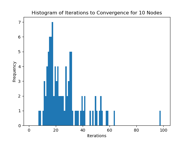
10 Nodes with 30% Edge Density
This works out to around: \[ 0.3 \times 10 \times 9 = 27 \text{ edges} \]
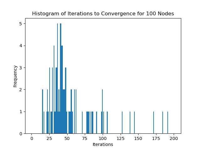
100 Nodes with 3% Edge Density
This works out to around: \[ 0.03 \times 100 \times 99 = 297 \text{ edges} \]
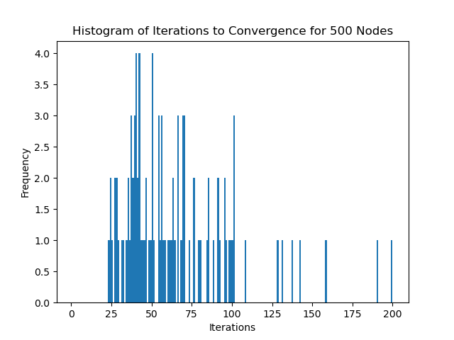
500 Nodes with 0.6% Edge Density
This works out to around:
\[
0.006 \times 500 \times 499 = 1497 \text{ edges}
\]
Observations
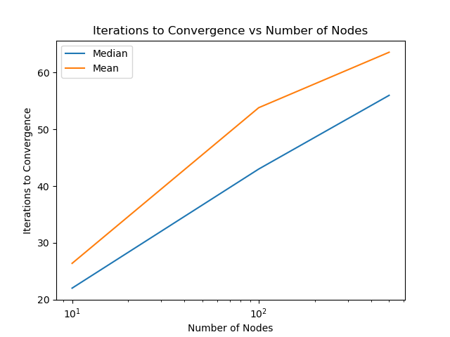
We see that in practice, the number of iterations required for convergence doesn't actually scale according to the number of edges in the graph. This is likely due to the fact that the complexity also depends on the maximum degree of the graph. In these examples, to not take too long, I've purposefully created sparser graphs as the number of nodes increases, which will decrease the maximum degree of the graph, keeping the number of iterations relatively constant despite the increase in the number of edges.
Conclusion
In this report, we've examined the multi-commodity flow problem and a localized solution method proposed by Liu et al. The method is intuitive and seems to produce good results in practice, scaling well with the number of edges in the graph, as long as the graph is sparse.
Furthermore, because of the parallelizable nature of the algorithm, it is possible to entirely offset the increase in computation time due to the increase in the number of edges by using more computational resources, calculating the height, congestion, and potential difference for each edge and node in parallel.
Further research could be done implement the algorithm in a more performant language such as C++ or Rust, and compare its performance with more standard mixed-integer programming solvers. This would give a better idea of the algorithm's performance in practice.
References
- Liu, P. A Localized Method for the Multi-commodity Flow Problem. arXiv:2108.07549 (2024). https://doi.org/10.48550/arXiv.2108.07549.
- He, B.S., Liao, L.Z. Improvements of Some Projection Methods for Monotone Nonlinear Variational Inequalities. Journal of Optimization Theory and Applications 112, 111–128 (2002). https://doi.org/10.1023/A:1013096613105.